If you've ever used JMeter, you know it's an awesome load testing tool. It also comes with a built-in graph listener, which allows you to watch JMeter do, well... something.
While this gives a basic view of response time and throughput, it doesn't show failures, nor how the server responds as load increases. And let's face it, it's just plain ugly.
Enter Matplotlib, a beautiful (though complex) plotting tool written in Python.
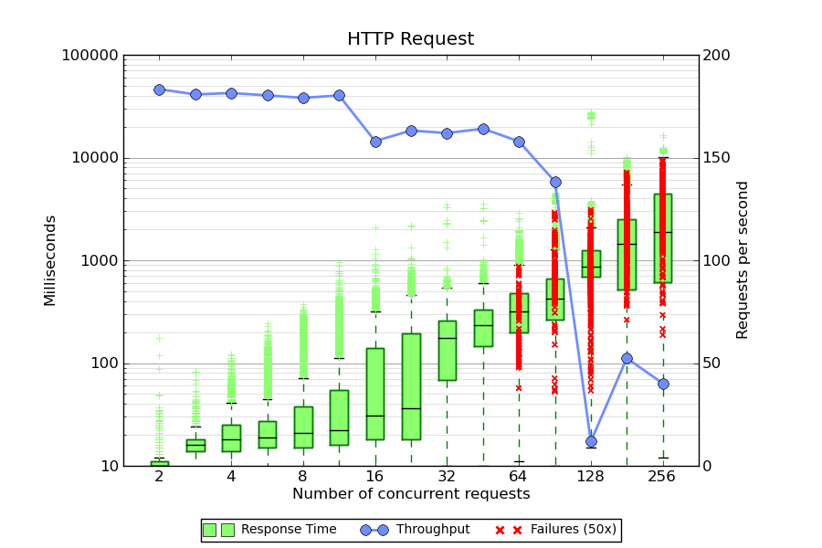
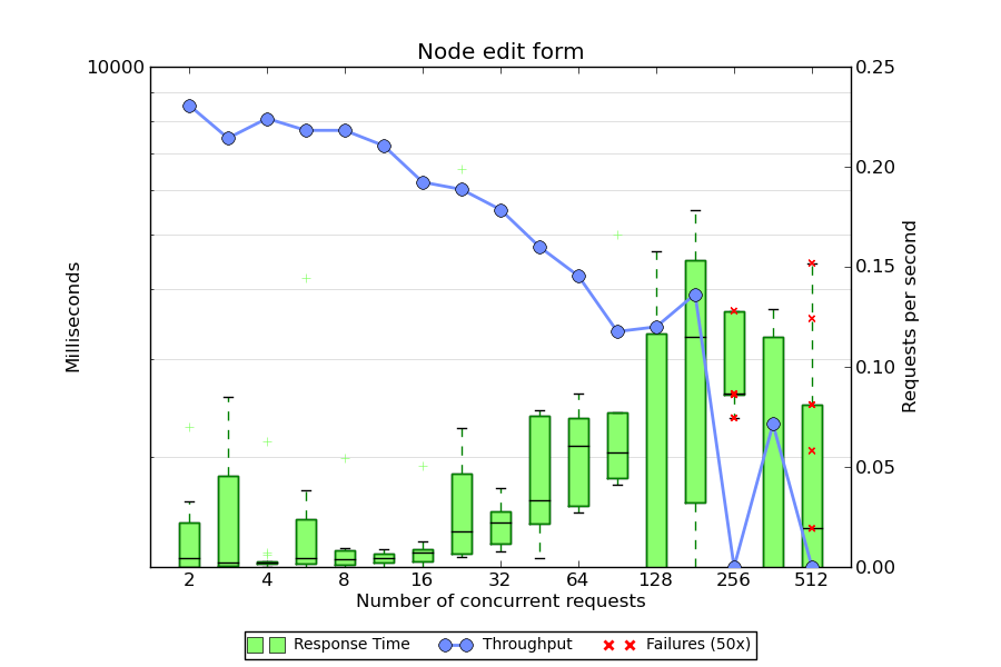
Box plots for response time are shown in green, throughput is in blue, and 50x errors are plotted as red X's. The script assumes a few things:
N-blah-blah.csv, where N is the number of threads. The file names are taken as command-line arguments.Stay tuned for the next article on the JMX file.
Click an image for a larger view.
#!/opt/local/bin/python2.6
# No copyright - https://creativecommons.org/publicdomain/zero/1.0/

from pylab import *
import numpy as na
import matplotlib.font_manager
import csv
import sys

elapsed = {}
timestamps = {}
starttimes = {}
errors = {}

# Parse the CSV files
for file in sys.argv[1:]:
  threads = int(file.split('-')[0])
  for row in csv.DictReader(open(file)):
    if (not row['label'] in elapsed):
      elapsed[row['label']] = {}
      timestamps[row['label']] = {}
      starttimes[row['label']] = {}
      errors[row['label']] = {}
    if (not threads in elapsed[row['label']]):
      elapsed[row['label']][threads] = []
      timestamps[row['label']][threads] = []
      starttimes[row['label']][threads] = []
      errors[row['label']][threads] = []
    elapsed[row['label']][threads].append(int(row['elapsed']))
    timestamps[row['label']][threads].append(int(row['timeStamp']))
    starttimes[row['label']][threads].append(int(row['timeStamp']) - int(row['elapsed']))
    if (row['success'] != 'true'):
      errors[row['label']][threads].append(int(row['elapsed']))

# Draw a separate figure for each label found in the results.
for label in elapsed:
  # Transform the lists for plotting
  plot_data = []
  throughput_data = [None]
  error_x = []
  error_y = []
  plot_labels = []
  column = 1
  for thread_count in sort(elapsed[label].keys()):
    plot_data.append(elapsed[label][thread_count])
    plot_labels.append(thread_count)
    test_start = min(starttimes[label][thread_count])
    test_end = max(timestamps[label][thread_count])
    test_length = (test_end - test_start) / 1000
    num_requests = len(timestamps[label][thread_count]) - len(errors[label][thread_count])
    if (test_length > 0):
      throughput_data.append(num_requests / float(test_length))
    else:
      throughput_data.append(0)
    for error in errors[label][thread_count]:
      error_x.append(column)
      error_y.append(error)
    column += 1


  # Start a new figure
  fig = figure(figsize=(9, 6))

  # Pick some colors
  palegreen = matplotlib.colors.colorConverter.to_rgb('#8CFF6F')
  paleblue = matplotlib.colors.colorConverter.to_rgb('#708DFF')

  # Plot response time
  ax1 = fig.add_subplot(111)
  ax1.set_yscale('log')
  bp = boxplot(plot_data, notch=0, sym='+', vert=1, whis=1.5)

  # Tweak colors on the boxplot
  plt.setp(bp['boxes'], color='g')
  plt.setp(bp['whiskers'], color='g')
  plt.setp(bp['medians'], color='black')
  plt.setp(bp['fliers'], color=palegreen, marker='+')

  # Now fill the boxes with desired colors
  numBoxes = len(plot_data)
  medians = range(numBoxes)
  for i in range(numBoxes):
    box = bp['boxes'][i]
    boxX = []
    boxY = []
    for j in range(5):
      boxX.append(box.get_xdata()[j])
      boxY.append(box.get_ydata()[j])
    boxCoords = zip(boxX,boxY)
    boxPolygon = Polygon(boxCoords, facecolor=palegreen)
    ax1.add_patch(boxPolygon)

  # Plot the errors
  if (len(error_x) > 0):
    ax1.scatter(error_x, error_y, color='r', marker='x', zorder=3)

  # Plot throughput
  ax2 = ax1.twinx()
  ax2.plot(throughput_data, 'o-', color=paleblue, linewidth=2, markersize=8)

  # Label the axis
  ax1.set_title(label)
  ax1.set_xlabel('Number of concurrent requests')
  ax2.set_ylabel('Requests per second')
  ax1.set_ylabel('Milliseconds')
  ax1.set_xticks(range(1, len(plot_labels) + 1, 2))
  ax1.set_xticklabels(plot_labels[0::2])
  fig.subplots_adjust(top=0.9, bottom=0.15, right=0.85, left=0.15)

  # Turn off scientific notation for Y axis
  ax1.yaxis.set_major_formatter(ScalarFormatter(False))

  # Set the lower y limit to the match the first column
  ax1.set_ylim(ymin=bp['boxes'][0].get_ydata()[0])

  # Draw some tick lines
  ax1.yaxis.grid(True, linestyle='-', which='major', color='grey')
  ax1.yaxis.grid(True, linestyle='-', which='minor', color='lightgrey')
  # Hide these grid behind plot objects
  ax1.set_axisbelow(True)

  # Add a legend
  line1 = Line2D([], [], marker='s', color=palegreen, markersize=10, linewidth=0)
  line2 = Line2D([], [], marker='o', color=paleblue, markersize=8, linewidth=2)
  line3 = Line2D([], [], marker='x', color='r', linewidth=0, markeredgewidth=2)
  prop = matplotlib.font_manager.FontProperties(size='small')
  figlegend((line1, line2, line3), ('Response Time', 'Throughput', 'Failures (50x)'),
    'lower center', prop=prop, ncol=3)

  # Write the PNG file
  savefig(label)